After four sold-out years in New York City, the R Conference made its debut in Washington DC to a sold-out crowd of data scientists at the Ronald Reagan Building on November 8th & 9th. Our speakers shared presentations on a variety of R-related topics.

A big thank you to our speakers Max Kuhn, Emily Robinson, Mike Powell, Mara Averick, Max Richman, Stephanie Hicks, Michael Garris, Kelly O’Briant, David Smith, Anna Kirchner, Roger Peng, Marck Vaisman, Soumya Kalra, Jonathan Hersh, Vivian Peng, Dan Chen, Catherine Zhou, Jim Klucar, Lizzy Huang, Refael Lav, Ami Gates, Abhijit Dasgupta, Angela Li  and Tommy Jones.

Some of the amazing speakers

Some highlights from the conference:

R Superstars Mara Averick, Roger Peng and Emily Robinson

Mara Averick, Roger Peng and Emily Robinson

A hallmark of our R conferences is that the speakers hang out with all the attendees and these three were crowd favorites.

Michael Powell Brings R to the aRmy

Major Michael Powell

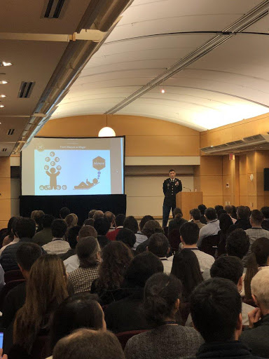
Major Michael Powell describes how R has brought efficiency to the Army Intelligence and Security Command by getting analysts out of Excel and into the Tidyverse. “Let me turn those 8 hours into 8 seconds for you,” says Powell.

Max Kuhn Explains the Applications of Equivocals to Apply Levels of Certainty to Predictions

Max Kuhn

After autographing his book, Applied Predictive Modeling, for a lucky attendee, Max Kuhn explains how Equivocals can be applied to individual predictions in order to avoid reporting predictions when there is significant uncertainty.

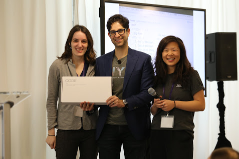
NYR and DCR Speaker Emily Robinson Getting an NYR Hoodie for her Awesome Tweeting

Emily Robinson

Emily Robinson tweeted the most at the 2018 NYR conference, winning her a WASD mechanical keyboard and at DCR she came in second so we gave her a limited edition NYR hoodie.

Max Richman Shows How SQL and R can Co-Exist

Max Richman

Max Richman, wearing the same shirt he wore when he spoke at the first NYR, shows parallels between dplyr and SQL.

Michael Garris Tells the Story of the MNIST Dataset

Michael Garris

Michael Garris was a member of the team that built the original MNIST dataset, which set the standard for handwriting image classification in the early 1990s. This talk may have been the first time the origin story was ever told.

R Stats Luminary Roger Peng Explains Relationship Between Air Pollution and Public Health

Roger Peng

Roger Peng shows us how air pollution levels has fallen over the past 50 years resulting in dramatic improvements in air quality and health (with help from R).

Kelly O’Briant Combining R with Serverless Computing

Kelly O'Briant

Kelly O’Briant demonstrates how to easily deploy R projects on Google Compute Engine and promoted the new #radmins hashtag.

Hot Dog vs Not Hot Dog by David Smith (Inspired by Jian-Yang from HBO’s Silicon Valley)

David Smith

David Smith, one of the original R users, shows how to recreate HBO’s Silicon Valley’s Not Hot Dog app using R and Azure

Jon Hersh Describes How to Push for Data Science Within Your Organization

Jon Hersh

Jon Hersh discusses the challenges, and solutions, of getting organizations to embrace data science.

Vivian Peng and the Importance of Data Storytelling

Vivian Peng

Vivian Peng asks the question, how do we protect the integrity of our data analysis when it’s published for the world to see?

Dan Chen Signs His Book for David Smith

Dan Chen and David Smith

Dan Chen autographing a copy of his book, Pandas for Everyone, for David Smith. Now David Smith has to sign his book, An Introduction to R, for Dan.

Malorie Hughes Analyzing Tweets

Malorie Hughes

On the first day I challenged the audience to analyze the tweets from the conference and Malorie Hughes, a data scientist with NPR, designed a Twitter analytics dashboard to track the attendee with the most tweets with the hashtag #rstatsdc. Seth Wenchel won a WASD keyboard for the best tweeting. And we presented Malorie wit a DCR speaker mug.

Strong Showing from the #RLadies!

The R-Ladies

The #rladies group is growing year after year and it is great seeing them in force at NYR and DCR!

Packages

Matthew Hendrickson, a DCR attendee, posted on twitter every package mentioned during the two-day conference: tidyverse, tidycensus, leaflet, leaflet.extras, funneljoin, glmnet, xgboost, rstan, rstanarm, LowRankQP, dplyr, coefplot, bayesplot, keras, tensorflow, lars, magrittr, purrr, rsample, useful, knitr, rmarkdown, ggplot2, ggiraph, ggrepel, ggraph, ggthemes, gganimate, ggmap, plotROC, ggridges, gtrendsr, tlnise, tm, Bioconductor, plyranges, sf, tmap, textmineR, tidytext, gmailr, rtweet, shiny, httr, parsnip, probably, plumber, reprex, crosstalk, arules and arulesviz.

Data Community DC

Data Community DC

A special thanks to the Data Community DC for helping us make the DC R Conference an incredible experience.

Videos

The videos for the conference will be posted in the coming weeks to dc.rstats.ai.

See You Next Year

Looking forward to more great conferences at next year’s NYR and DCR!

Related Posts


Jared Lander is the Chief Data Scientist of Lander Analytics a New York data science firm, Adjunct Professor at Columbia University, Organizer of the New York Open Statistical Programming meetup and the New York and Washington DC R Conferences and author of R for Everyone.

Getting People Started

A large part of my work is teaching R–for private clients, at Columbia Business School, at conferences and facilitating public workshops for others.

A common theme is that getting everyone setup on their individual computers is very difficult. No matter how many instructions I provide, there are always a good number of people without a proper environment. This can mean not using RStudio projects, not having the right packages installed, not downloading the data and sometimes not even installing R.

Solution

After many experiments I finally came upon a solution. For every class I teach I now create a skeleton project hosted on GitHub with instructions for setup.

The instructions (in the README) consist of three blocks of code.

  1. Package installation
  2. Copying the project structure from the repo (no git required)
  3. Downloading data

All the user has to do is copy and paste these three blocks of code into the R console and they have the exact same environment as the instructor and other students.

packages <- c( 
    'coefplot', 
    'rprojroot', 
    'tidyverse', 
    'usethis'
)
install.packages(packages)
newProject <- usethis::use_course('https://github.com/jaredlander/WorkshopExampleRepo/archive/master.zip')
source('prep/DownloadData.r')

Using this process, 95% of my students are prepared for class.

The inspiration for this idea came from a fun coffee with Hadley Wickham and Jenny Bryan during a conference in New Zealand and the implementation is made possible thanks to the usethis package.

Automating the Setup

Now that I found a good way to get students started, I wanted to make it easier for me to setup the repo. So I created an R package called RepoGenerator and put it on CRAN.

The first step to using the package is to create a GitHub Personal Access Token (instructions are in the README). Then you build a data.frame listing datasets you want the students to download. The data.frame needs at least the following three columns.

  • Local: The name, not path, the file should have on disk
  • Remote: The URL where the data files are stored online
  • Mode: The mode needed to write the file to disk, ‘w’ for regular text files, ‘wb’ for binary files such as Excel or rds files

An example data.frame is available in the RepoGenerator package.

data(datafiles, package='RepoGenerator')
datafiles[1:6, c('Local', 'Remote', 'Mode')]

After that you define the packages you want your students to use. There can be as few or as many as you want. In addition to any packages you list, rprojroot and usethis are added so that the instructions in the new repo will be certain to work.

packages <- c('caret', 'coefplot','DBI', 'dbplyr', 'doParallel', 'dygraphs', 
              'foreach', 'ggthemes', 'glmnet', 'jsonlite', 'leaflet', 'odbc', 
              'recipes', 'rmarkdown', 'rprojroot', 'RSQLite', 'rvest', 
              'tidyverse', 'threejs', 'usethis', 'UsingR', 'xgboost', 'XML', 
              'xml2')

Now all you need to do is call the createRepo() function.

createRepo(
    # the name to use for the repo and project
    name='WorkshopExampleRepo', 
    # the location on disk to build the project
    path='~/WorkshopExampleRepo',
    # the data.frame listing data files for the user to download
    data=datafiles,
    # vector of packages the user should install
    packages=packages,
    # the GitHub username to create the repo for
    user='jaredlander',
    # the new repo's README has the name of who is organizing the class
    organizer='Lander Analytics',
    # the name of the environment variable storing the GitHub Personal Access Token
    token='MyGitHubPATEnvVar'
)

After this you will have a new repo setup for your users to copy, including instructions.

That’s All

Reducing setup issues at the start of a training can really improve the experience for everyone and allow you to get straight into teaching.

Please check it out and let me know how it works for you.


Related Posts


Jared Lander is the Chief Data Scientist of Lander Analytics a New York data science firm, Adjunct Professor at Columbia University, Organizer of the New York Open Statistical Programming meetup and the New York and Washington DC R Conferences and author of R for Everyone.

2018 New York R Conference

The 2018 New York R Conference was the biggest and best yet. This is both in terms of the crowd size and content.  The speakers included some of the R community’s best such as Hadley Wickham, David Robinson, Jennifer Hill, Max Kuhn, Andreas Mueller (ok, a little Python), Evelina Gabasova, Sean Taylor and Jeff Ryan. I am proud to say we were almost at gender parity for both attendees and speakers which is amazing for a tech conference. Brooke Watson even excitedly noted that we had a line for the women’s room.

Particularly gratifying for me was seeing so many of my students speak. Eurry Kim, Dan Chen and Alex Boghosian all gave excellent talks.

Some highlights that stuck out to me are:

Emily Robinson Shows There is More to the Tidyverse than Hadley

The Expanded Tidyverse

Emily Robinson, otherwise known as ERob, gave an excellent talk showing how the Tidyverse is so much more than just Hadley and that there are many people inspired by him to contribute in the Tidy way.

Sean Taylor Forecasted the Future with Prophet

Sean Taylor

Sean Taylor, former New Yorker and unrepentant Eagles fan, demonstrate his powerful R and Python, package Prophet, for forecasting time series data. Facebook open sourced his work so we could all benefit.

OG Data Mafia Founder Drew Conway Popped In

Giving away a data mafia shirt

A lucky fan got an autographed NYC Data Mafia t-shirt from Drew Conway.

David Smith Playing Minecraft Through R

Minecraft in R

David Smith played Minecraft through R, including building objects and moving through the world.

Evelina Gabasova Used Social Network Analysis to Break Down Star Wars

It's a Trap

Evelina Gabasova wowed the audience with her fun talk and detailed analysis of character interaction in Star Wars.

Dusty Turner Represented West Point

Dusty Talking Army Sports

Dusty Turner taught us how the United States Military Academy uses R for both student instruction and evaluation.

Hadley Wickham Delved into the Nitty Gritty of R

Hadley shows off objects are stored in memory

Hadley Wickham showed us how to get into the internals of R and figure out how to examine objects from a memory perspective.

Jennifer Hill Demonstrated Awesome Machine Learning Techniques for Causal Inference

Jennifer Hill Explaining Causal Inference

Following her sold-out meetup appearance in March, Jennifer continued to push the boundaries of causal inference.

I Made the Authors of Caret and scitkit-learn Show That R and Python Can Get Along

Caret and Scikit-learn in one place

While both Andreas and Max gave great individual talks, I made them pose for this peace-making photo.

David Robinson Got the Upper Hand in a Sibling Twitter Duel

DRob Teaching

Given only about 30 minutes notice, David put together an entire slideshow on how to livetweet and how to compete with your sibling.

In the End Emily Robinson Beat Her Brother For Best Tweeting

Emily won the prize for best tweeting

Despite David’s headstart Emily was the best tweeter (as calculated by Max Kuhn and Mara Averick) so she won the WASD Code mechanical keyboard with MX Cherry Clear switches.

Silent Auction of Data Paintings

The Robinson Family bought the Pizza Data painting for me

Thomas Levine made paintings of famous datasets that we auctioned off with the proceeds supporting the R Foundation and the Free Software Foundation. The Robinson family very graciously chipped in and bought the painting of the Pizza Poll data for me! I’m still floored by this and in love with the painting.

Ice Cream Sandwiches

Ice Cream Sandwiches

In addition to bagels and eggs sandwiches from Murray’s Bagels, Israeli food from Hummus and Pita Company, avocado toast and coffee from Bluestone Lane Coffee and pizza from Fiore’s, we also had ice creams sandwiches from World’s Best Cookie Dough.

All the Material

To catch up on all the presentations check out Mara Averick’s excellent notes:

Or check out all of Brooke’s drawings, collated by Dan Chen.

Videos and Upcoming Events

The videos will be posted at rstats.nyc in a few weeks for all to enjoy.

There are a number of other events coming up including:

We are already beginning plans for next year’s conference and are working on bringing it to DC as well! Stay tuned for all that and more.

Dan loves his mug

Related Posts


Jared Lander is the Chief Data Scientist of Lander Analytics a New York data science firm, Adjunct Professor at Columbia University, Organizer of the New York Open Statistical Programming meetup and the New York and Washington DC R Conferences and author of R for Everyone.

In my last post I discussed using coefplot on glmnet models and in particular discussed a brand new function, coefpath, that uses dygraphs to make an interactive visualization of the coefficient path.

Another new capability for version 1.2.5 of coefplot is the ability to show coefficient plots from xgboost models. Beyond fitting boosted trees and boosted forests, xgboost can also fit a boosted Elastic Net. This makes it a nice alternative to glmnet even though it might not have some of the same user niceties.

To illustrate, we use the same data as our previous post.

First, we load the packages we need and note the version numbers.

# list the packages that we load
# alphabetically for reproducibility
packages <- c('caret', 'coefplot', 'DT', 'xgboost')
# call library on each package
purrr::walk(packages, library, character.only=TRUE)

# some packages we will reference without actually loading
# they are listed here for complete documentation
packagesColon <- c('dplyr', 'dygraphs', 'knitr', 'magrittr', 'purrr', 'tibble', 'useful')
versions <- c(packages, packagesColon) %>% 
    purrr::map(packageVersion) %>% 
    purrr::map_chr(as.character)
packageDF <- tibble::data_frame(Package=c(packages, packagesColon), Version=versions) %>% 
    dplyr::arrange(Package)
knitr::kable(packageDF)
Package Version
caret 6.0.78
coefplot 1.2.6
dplyr 0.7.4
DT 0.2
dygraphs 1.1.1.4
knitr 1.18
magrittr 1.5
purrr 0.2.4
tibble 1.4.2
useful 1.2.3
xgboost 0.6.4

Then, we read the data. The data are available at https://www.jaredlander.com/data/manhattan_Train.rds with the CSV version at data.world. We also get validation data which is helpful when fitting xgboost mdoels.

manTrain <- readRDS(url('https://www.jaredlander.com/data/manhattan_Train.rds'))
manVal <- readRDS(url('https://www.jaredlander.com/data/manhattan_Validate.rds'))

The data are about New York City land value and have many columns. A sample of the data follows. There’s an odd bug where you have to click on one of the column names for the data to display the actual data.

datatable(manTrain %>% dplyr::sample_n(size=1000), elementId='TrainingSampled',
              rownames=FALSE,
              extensions=c('FixedHeader', 'Scroller'),
              options=list(
                  scroller=TRUE
              ))

While glmnet automatically standardizes the input data, xgboost does not, so we calculate that manually. We use preprocess from caret to compute the mean and standard deviation of each numeric column then use these later.

preProc <- preProcess(manTrain, method=c('center', 'scale'))

Just like with glmnet, we need to convert our tbl into an X (predictor) matrix and a Y (response) vector. Since we don’t have to worry about multicolinearity with xgboost we do not want to drop the baselines of factors. We also take advantage of sparse matrices since that reduces memory usage and compute, even though this dataset is not that large.

In order to build the matrix and vector we need a formula. This could be built programmatically, but we can just build it ourselves. The response is TotalValue.

valueFormula <- TotalValue ~ FireService + ZoneDist1 + ZoneDist2 +
    Class + LandUse + OwnerType + LotArea + BldgArea + ComArea + ResArea +
    OfficeArea + RetailArea + NumBldgs + NumFloors + UnitsRes + UnitsTotal + 
    LotDepth + LotFront + BldgFront + LotType + HistoricDistrict + Built + 
    Landmark
manX <- useful::build.x(valueFormula, data=predict(preProc, manTrain),
                        # do not drop the baselines of factors
                        contrasts=FALSE,
                        # use a sparse matrix
                        sparse=TRUE)

manY <- useful::build.y(valueFormula, data=manTrain)

manX_val <- useful::build.x(valueFormula, data=predict(preProc, manVal),
                        # do not drop the baselines of factors
                        contrasts=FALSE,
                        # use a sparse matrix
                        sparse=TRUE)

manY_val <- useful::build.y(valueFormula, data=manVal)

There are two functions we can use to fit xgboost models, the eponymous xgboost and xgb.train. When using xgb.train we first store our X and Y matrices in a special xgb.DMatrix object. This is not a necessary step, but makes things a bit cleaner.

manXG <- xgb.DMatrix(data=manX, label=manY)
manXG_val <- xgb.DMatrix(data=manX_val, label=manY_val)

We are now ready to fit a model. All we need to do to fit a linear model instead of a tree is set booster='gblinear' and objective='reg:linear'.

mod1 <- xgb.train(
    # the X and Y training data
    data=manXG,
    # use a linear model
    booster='gblinear',
    # minimize the a regression criterion 
    objective='reg:linear',
    # use MAE as a measure of quality
    eval_metric=c('mae'),
    # boost for up to 500 rounds
    nrounds=500,
    # print out the eval_metric for both the train and validation data
    watchlist=list(train=manXG, validate=manXG_val),
    # print eval_metric every 10 rounds
    print_every_n=10,
    # if the validate eval_metric hasn't improved by this many rounds, stop early
    early_stopping_rounds=25,
    # penalty terms for the L2 portion of the Elastic Net
    lambda=10, lambda_bias=10,
    # penalty term for the L1 portion of the Elastic Net
    alpha=900000000,
    # randomly sample rows
    subsample=0.8,
    # randomly sample columns
    col_subsample=0.7,
    # set the learning rate for gradient descent
    eta=0.1
)
## [1]  train-mae:1190145.875000    validate-mae:1433464.750000 
## Multiple eval metrics are present. Will use validate_mae for early stopping.
## Will train until validate_mae hasn't improved in 25 rounds.
## 
## [11] train-mae:938069.937500 validate-mae:1257632.000000 
## [21] train-mae:932016.625000 validate-mae:1113554.625000 
## [31] train-mae:931483.500000 validate-mae:1062618.250000 
## [41] train-mae:931146.750000 validate-mae:1054833.625000 
## [51] train-mae:930707.312500 validate-mae:1062881.375000 
## [61] train-mae:930137.375000 validate-mae:1077038.875000 
## Stopping. Best iteration:
## [41] train-mae:931146.750000 validate-mae:1054833.625000

The best fit was arrived at after 41 rounds. We can see how the model did on the train and validate sets using dygraphs.

dygraphs::dygraph(mod1$evaluation_log)

We can now plot the coefficients using coefplot. Since xgboost does not save column names, we specify it with feature_names=colnames(manX). Unlike with glmnet models, there is only one penalty so we do not need to specify a specific penalty to plot.

coefplot(mod1, feature_names=colnames(manX), sort='magnitude')

This is another nice addition to coefplot utilizing the power of xgboost.

Related Posts


Jared Lander is the Chief Data Scientist of Lander Analytics a New York data science firm, Adjunct Professor at Columbia University, Organizer of the New York Open Statistical Programming meetup and the New York and Washington DC R Conferences and author of R for Everyone.

I’m a big fan of the Elastic Net for variable selection and shrinkage and have given numerous talks about it and its implementation, glmnet. In fact, I will even have a DataCamp course about glmnet coming out soon.

As a side note, I used to pronounce it g-l-m-net but after having lunch with one of its creators, Trevor Hastie, I learn it is pronounced glimnet.

coefplot has long supported glmnet via a standard coefficient plot but I recently added some functionality, so let’s take a look. As we go through this, please pardon the htmlwidgets in iframes.

First, we load packages. I am now fond of using the following syntax for loading the packages we will be using.

# list the packages that we load
# alphabetically for reproducibility
packages <- c('coefplot', 'DT', 'glmnet')
# call library on each package
purrr::walk(packages, library, character.only=TRUE)

# some packages we will reference without actually loading
# they are listed here for complete documentation
packagesColon <- c('dplyr', 'knitr', 'magrittr', 'purrr', 'tibble', 'useful')

The versions can then be displayed in a table.

versions <- c(packages, packagesColon) %>% 
    purrr::map(packageVersion) %>% 
    purrr::map_chr(as.character)
packageDF <- tibble::data_frame(Package=c(packages, packagesColon), Version=versions) %>% 
    dplyr::arrange(Package)
knitr::kable(packageDF)
Package Version
coefplot 1.2.5.1
dplyr 0.7.4
DT 0.2
glmnet 2.0.13
knitr 1.18
magrittr 1.5
purrr 0.2.4
tibble 1.4.1
useful 1.2.3

First, we read some data. The data are available at https://www.jaredlander.com/data/manhattan_Train.rds with the CSV version at data.world.

manTrain <- readRDS(url('https://www.jaredlander.com/data/manhattan_Train.rds'))

The data are about New York City land value and have many columns. A sample of the data follows.

datatable(manTrain %>% dplyr::sample_n(size=100), elementId='DataSampled',
              rownames=FALSE,
              extensions=c('FixedHeader', 'Scroller'),
              options=list(
                  scroller=TRUE,
                  scrollY=300
              ))

In order to use glmnet we need to convert our tbl into an X (predictor) matrix and a Y (response) vector. Since we don’t have to worry about multicolinearity with glmnet we do not want to drop the baselines of factors. We also take advantage of sparse matrices since that reduces memory usage and compute, even though this dataset is not that large.

In order to build the matrix ad vector we need a formula. This could be built programmatically, but we can just build it ourselves. The response is TotalValue.

valueFormula <- TotalValue ~ FireService + ZoneDist1 + ZoneDist2 +
    Class + LandUse + OwnerType + LotArea + BldgArea + ComArea + ResArea +
    OfficeArea + RetailArea + NumBldgs + NumFloors + UnitsRes + UnitsTotal + 
    LotDepth + LotFront + BldgFront + LotType + HistoricDistrict + Built + 
    Landmark - 1

Notice the - 1 means do not include an intercept since glmnet will do that for us.

manX <- useful::build.x(valueFormula, data=manTrain,
                        # do not drop the baselines of factors
                        contrasts=FALSE,
                        # use a sparse matrix
                        sparse=TRUE)

manY <- useful::build.y(valueFormula, data=manTrain)

We are now ready to fit a model.

mod1 <- glmnet(x=manX, y=manY, family='gaussian')

We can view a coefficient plot for a given value of lambda like this.

coefplot(mod1, lambda=330500, sort='magnitude')

A common plot that is built into the glmnet package it the coefficient path.

plot(mod1, xvar='lambda', label=TRUE)

This plot shows the path the coefficients take as lambda increases. They greater lambda is, the more the coefficients get shrunk toward zero. The problem is, it is hard to disambiguate the lines and the labels are not informative.

Fortunately, coefplot has a new function in Version 1.2.5 called coefpath for making this into an interactive plot using dygraphs.

coefpath(mod1)

While still busy this function provides so much more functionality. We can hover over lines, zoom in then pan around.

These functions also work with any value for alpha and for cross-validated models fit with cv.glmnet.

mod2 <- cv.glmnet(x=manX, y=manY, family='gaussian', alpha=0.7, nfolds=5)

We plot coefficient plots for both optimal lambdas.

# coefplot for the 1se error lambda
coefplot(mod2, lambda='lambda.1se', sort='magnitude')

# coefplot for the min error lambda
coefplot(mod2, lambda='lambda.min', sort='magnitude')

The coefficient path is the same as before though the optimal lambdas are noted as dashed vertical lines.

coefpath(mod2)

While coefplot has long been able to plot coefficients from glmnet models, the new coefpath function goes a long way in helping visualize the paths the coefficients take as lambda changes.

Related Posts


Jared Lander is the Chief Data Scientist of Lander Analytics a New York data science firm, Adjunct Professor at Columbia University, Organizer of the New York Open Statistical Programming meetup and the New York and Washington DC R Conferences and author of R for Everyone.