About Jared

hates carrots and loves visiting nursing homes in a pedobear costume

This year’s Pi Cake courtesy of Chrissie Cook:

Side View:

And don’t forget this is Albert Einstein’s birthday was well.

How are you celebrating this fantastic geek holiday?

Like last year, the NYC Data Mafia will be out celebrating with (round) pizza.

Related Posts


Jared Lander is the Chief Data Scientist of Lander Analytics a New York data science firm, Adjunct Professor at Columbia University, Organizer of the New York Open Statistical Programming meetup and the New York and Washington DC R Conferences and author of R for Everyone.

Shortly after the Giants fantastic defeat of the Patriots in Super Bowl XLVI (I was a little disappointed that Eli, Coughlin and the Vince Lombardi Trophy all got off the parade route early and the views of City Hall were obstructed by construction trailers, but Steve Weatherford was awesome as always) a friend asked me to settle a debate amongst some people in a Super Bowl pool.

He writes:

We have 10 participants in a superbowl pool.  The pool is a “pick the player who scores first” type pool.  In a hat, there are 10 Giants players.  Each participant picks 1 player out of the hat (in no particular order) until the hat is emptied.  Then 10 Patriots players go in the hat and each participant picks again.

In the end, each of the 10 participants has 1 Giants player and 1 Patriots player.  No one has any duplicate players as 10 different players from each team were selected.  Pool looks as follows:

Participant 1 Giant A Patriot Q
Participant 2 Giant B Patriot R
Participant 3 Giant C Patriot S
Participant 4 Giant D Patriot T
Participant 5 Giant E Patriot U
Participant 6 Giant F Patriot V
Participant 7 Giant G Patriot W
Participant 8 Giant H Patriot X
Participant 9 Giant I Patriot Y
Participant 10 Giant J Patriot Z

Winners = First Player to score wins half the pot.  First player to score in 2nd half wins the remaining half of the pot.

The question is, what are the odds that someone wins Both the 1st and 2nd half.  Remember, the picks were random.

Before anyone asks about the safety, one of the slots was for Special Teams/Defense.

There are two probabilistic ways of thinking about this.  Both hinge on the fact that whoever scores first in each half is both independent and not mutually exclusive.

First, let’s look at the two halves individually.  In a given half any of 20 players can score first (10 from the Giants and 10 from the Patriots) and an individual participant can win with two of those.  So a participant has a 2/20 = 1/10 chance of winning a half.  Thus that participant has a (1/10) * (1/10) = 1/100 chance of winning both halves.  Since there are 10 participants there is an overall probability of 10 * (1/100) = 1/10 of any single participant winning both halves.

The other way is to think a little more combinatorically.  There are 20 * 20 = 400 different combinations of players scoring first in each half.  A participant has two players which are each valid for each half giving them four of the possible combinations leading to a 4 / 400 = 1/100 probability that a single participant will win both halves.  Again, there are 10 participants giving an overall 10% chance of any one participant winning both halves.

Since both methods agreed I am pretty confidant in the results, but just in case I ran some simulations in R which you can find after the break.

Continue reading

Related Posts


Jared Lander is the Chief Data Scientist of Lander Analytics a New York data science firm, Adjunct Professor at Columbia University, Organizer of the New York Open Statistical Programming meetup and the New York and Washington DC R Conferences and author of R for Everyone.

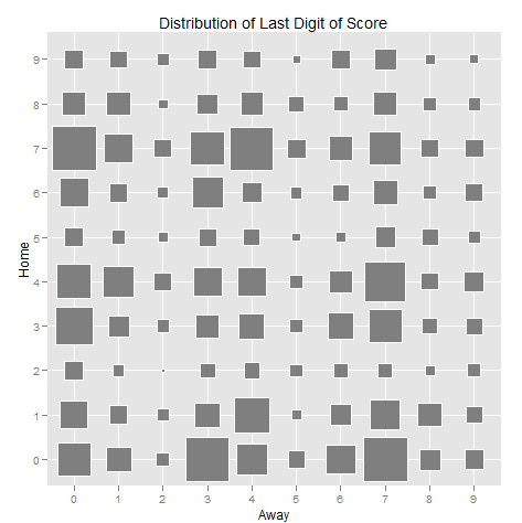
With the Super Bowl only hours away now is your last chance to buy your boxes.  Assuming the last digits are not assigned randomly you can maximize your chances with a little analysis.  While I’ve seen plenty of sites giving the raw numbers, I thought a little visualization was in order.

In the graph above (made using ggplot2 in R, of course) the bigger squares represent greater frequency.  The axes are labelled “Home” and “Away” for orientation, but in the Super Bowl that probably doesn’t matter too much, especially considering that Indianapolis is (Peyton) Manning territory so the locals will most likely be rooting for the Giants.  Further, I believe Super Bowl XLII, featuring the same two teams, had a disproportionate number of Giants fans.  Bias disclaimer:  GO BIG BLUE!!!

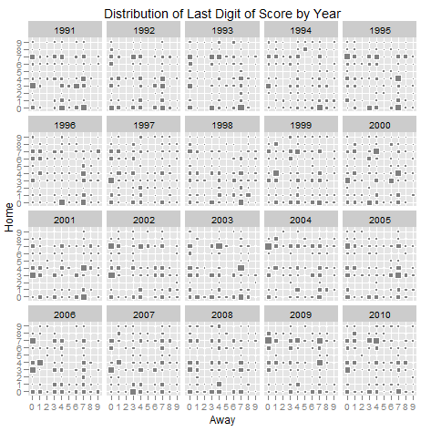
Below is the same graph broken down by year to see how the distribution has changed over the past 20 years.

All the data was scraped from Pro Football Reference.  All of my code and other graphs that didn’t make the cut are at my github site.

As always, send any questions my way.

Related Posts


Jared Lander is the Chief Data Scientist of Lander Analytics a New York data science firm, Adjunct Professor at Columbia University, Organizer of the New York Open Statistical Programming meetup and the New York and Washington DC R Conferences and author of R for Everyone.

Taking a break from my normal exposition on stats, New York or pizza I’d like to espouse the wonders of baking soda and vinegar!

My sink was clogged, not with anything specific, but just years worth of gunk.  So after scraping out what I could with my hands and a wire hanger–and wanting to avoid caustic chemicals like Drano–I searched the Internet to see if Listerene or Coca-Cola might do the trick.  But extensive searching led me to baking soda and vinegar.

It’s very simple:  Stuff a half cup of baking soda into the train then pour a half cup of vinegar down it, return the sink stopper and wait 15 minutes.  Then pour down another half cup of vinegar, close the stopper and wait another 15 minutes.  After that pour a gallon (a tea kettle’s worth) of boiling water down the drain and you’re done!  Not only will it unclog your drain, it leaves all the chrome shining like new!

For those of us who never got to make a model volcano in science class it was really awesome watching the baking soda and vinegar react

Related Posts


Jared Lander is the Chief Data Scientist of Lander Analytics a New York data science firm, Adjunct Professor at Columbia University, Organizer of the New York Open Statistical Programming meetup and the New York and Washington DC R Conferences and author of R for Everyone.

A new study, reported in the New York Times, tracked population movements in post-earthquake Haiti using cell phone data.  The article grabbed my attention because one of the authors, Richard Garfield (whom I have done numerous projects with and who has his own Wikipedia entry!), had told me about this very study just a few months ago.

Over dinner in New York’s Little India he explained how the largest cell phone company in Haiti provided him with anonymized cell tower records.  As many people are aware, cell phones–even those without GPS–report their locations back to cell towers at regular intervals.  By tracking the daily position of the phones before and after the earthquake they were able to determine that 20% of Port-Au-Prince’s population had left the capitol within 19 days of the disaster.

They used plenty of solid math in the analysis and amazingly did it all without resorting to spatial statistics.  They have some nice map-based visualizations but I’ve been meaning to get the data from Dr. Garfield so I can attempt something similar to the amazing work done by the NYC Data Mafia on the WikiLeaks Afghanistan data.  Though I don’t promise anything nearly as good.

It is also worth noting that they did this at a fraction of the cost and time of an extensive UN survey.  That survey only had about 2,500 respondents whereas the cell phone project incorporated around 1.9 million people without them spending valuable time with an interviewer.

Related Posts


Jared Lander is the Chief Data Scientist of Lander Analytics a New York data science firm, Adjunct Professor at Columbia University, Organizer of the New York Open Statistical Programming meetup and the New York and Washington DC R Conferences and author of R for Everyone.


While playing Words with Friends my randomly chosen opponent played “radiale” as her first word.  Since that used up all of her tiles, she received a bonus on top of all the points the word itself got, resulting in a one-move score of 53 points!  Rather than being impressed I was upset at the large deficit I would have to overcome.

To combat this I did what comes naturally:  Write an R script to find the perfect word!

Needing to combine my seven letters with one of her letters there were two routes I could take.  The first would be for each combination of my seven letters and one of hers, find all 40,320 (8!) permutations then hit dictionary.com to see if it is a real word for a total of 282,240 (8!*7) http calls.  That seemed a bit excessive and impractical so I moved on to the next idea.

So, first thing I did was pull a list of common eight-letter words. Then for each combination of my letters and one of hers (only 7 iterations) I checked if those letters (in any order) matched the letters in any of the possible words.  Once a match was found there was a check for the counts of the letters and if that passed then the word was recorded as a true match.

The algorithm took about 17 seconds to run and found me one possible word for my letters combined with one of hers:  “headrace”, for 63 points!  Perhaps I should have been able to figure that out on my own, but where would be the fun in that.  Find the code after the break.

Related Posts


Jared Lander is the Chief Data Scientist of Lander Analytics a New York data science firm, Adjunct Professor at Columbia University, Organizer of the New York Open Statistical Programming meetup and the New York and Washington DC R Conferences and author of R for Everyone.

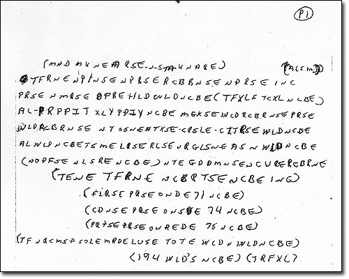
The FBI has put out a public request for help cracking a code.  The code above was found in the pants of a murder victim over 10 years ago.  Despite some of the best code breakers in the world give it a shot, they have not been able to break the code.  I wonder if the NSA had a go at it.  Couldn’t they try brute force like in Dan Brown’s Digital Fortress?  Yes I referenced Dan Brown in the same paragraph as the NSA, deal with it.

If you think you can help send a letter to:

FBI Laboratory
Cryptanalysis and Racketeering Records Unit
2501 Investigation Parkway
Quantico, VA 22135
Attn: Ricky McCormick Case

There’s no reward but you’d be helping your country.

Related Posts


Jared Lander is the Chief Data Scientist of Lander Analytics a New York data science firm, Adjunct Professor at Columbia University, Organizer of the New York Open Statistical Programming meetup and the New York and Washington DC R Conferences and author of R for Everyone.

Pi Day Celebrants

As mentioned earlier, yesterday was Pi Day so a bunch of statisticians and other such nerds celebrated at the new(ish) Artichoke Basille near the High Line.  We had three pies:  the signature Artichoke, the Margherita and the Anchovy, which was delicious but only some of us ate.  And of course we had our custom cake from Chrissie Cook.

The photos were taken by John.

Pi Cake 2011
NYC Data Mafia
NYC Data Mafia

Related Posts


Jared Lander is the Chief Data Scientist of Lander Analytics a New York data science firm, Adjunct Professor at Columbia University, Organizer of the New York Open Statistical Programming meetup and the New York and Washington DC R Conferences and author of R for Everyone.

Pi CakeHappy Pi Day everybody!  I’ll be out celebrating with the rest of the NYC Data Mafia eating pizza and devouring the above Pi Cake, custom baked by Chrissie Cook.

Today is also Albert Einstein’s birthday so there are plenty of reasons to have fun.

The cake below was my first ever Pi Cake in what is sure to become an annual tradition.

Pi Cake 2009

Update: Drew Conway does far more justice to our fair, irrational, transcendental number.

Update 2:  Engadget posted this awesome video of “What Pi Sounds Like.

Related Posts


Jared Lander is the Chief Data Scientist of Lander Analytics a New York data science firm, Adjunct Professor at Columbia University, Organizer of the New York Open Statistical Programming meetup and the New York and Washington DC R Conferences and author of R for Everyone.
This graphs shows received and sent texts by month.  Notice the spike in July 2010.
Fig. 1: This graph shows received and sent text messages by month. Notice the spike in July 2010.

A few weeks ago my iPhone for some reason erased ALL of my previous text messages (SMS and MMS) and it was as if I was starting with a new phone. After doing some digging I discovered that each time you sync your iPhone a copy of its text message database is saved on your computer which can be accessed without jailbreaking.

My original intent was to take the old database and union it with the new database for all the texting I had done since then, thus restoring all of my text messages. But once I got into the SQLite database I realized that I had a ton of information on my hands that was begging to be analyzed. It also didn’t hurt that I was in a lovely but small Vermont town for the week without much else to do at night.

My first finding, as seen above, is that my text messaging spiked after my girlfriend and I broke up around July of last year. Notice that for both years there is a dip in December. That’s because in 2009 I was in Burma during December and for 2010 the data stopped on December 6th when the last backup was made. A simple t-test confirmed that my texting did indeed increase after the breakup.

Fig. 2: This graph shows my text messaging pattern over time for both men and women. Notice the crossover around August 2010.

More interestingly, is that before my girlfriend and I broke up last year I texted more men than women, but shortly after we broke up that flipped. I don’t think that needs much of an explanation. The above graph and further analysis excludes her and family members because they would bias the gender effect. Being a good statistician I ran a poisson regression to see if there really was a significant change. The coefficient plot below (which is on the logarithmic scale) shows that my texting with males increased after the breakup (or Epoch) by 74% (calculated by summing the coefficients for “Epoch”, “Male” and “Male:Epoch” and then exponentiating) while my texting with females increased 127%.

Fig. 3: Here the “Male” coefficient seems statistically insignificant but its direction makes sense so it is left in the model. The “Intercept” is interpreted as the texting rate with females before the breakup, “Epoch” is the increase with females after the breakup, “Intercept” plus “Male” is the rate with males before the breakup. “Epoch” combined with “Male:Epoch” is the change in rate for texts with males after the breakup.

Further analysis and a how-to after the break.

Continue reading

Related Posts


Jared Lander is the Chief Data Scientist of Lander Analytics a New York data science firm, Adjunct Professor at Columbia University, Organizer of the New York Open Statistical Programming meetup and the New York and Washington DC R Conferences and author of R for Everyone.